Pothole Detection using Computer Vision (AI Tool)

 In this blog, we cover pothole detection designing using the Matlab computer vision toolbox. Potholes are road defects that are caused by depression in road surfaces during wet seasons and heavy traffics. Fiji roads are susceptible to potholes due to the weather pattern and heavy traffics.  One of the most persistent issues is the prevalence of potholes, which can cause accidents and damage to vehicles. 

The pothole detection model is compromised with strategies that enveloped a complete functional model. However, as there are various existing pre-trained models that have already existed, we will try to train and perform some comparisons among these state-of-arts.

1. Yolov2
2. Yolov3
3. Fast RCNN
4. Faster RCNN

Methods followed for training a Pothole Detection model

The strategies taken to train a Pothole Detection involve other sub-strategies that are necessary to take before feeding data into a neural-based model.

Fig 1: Task Execution Flow

Image Labeling

Image Labelling is the process of creating bounding boxes around the pothole to create a region of interest (ROI) for the model to focus on. It is smart to keep the ROI as tight as possible to the pothole to avoid confusion and misclassification of incorrect localization.

Data Augmentation

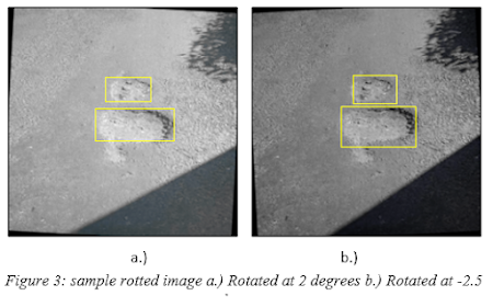
Data augmentation is a technique of twisting the image representation to allow the model to pick the different possible features from the same image. It represents the image with different orientations, light intensities, and conditions to the model. It also expands the data size by representing an image multiple times with different features. The following argumentation transformations were performed on each input image, where all augmentation techniques are available as a generic custom function file on Matlab.

The images in Fig 2 express the following augmentation techniques.

        a.) Color jitter augmentation in HSV space

        b.) Random horizontal flip

        c.) Grayscale

        d.) Random scaling by 10 percent

The following conditions were set for jitter augmentation in HSV space.

1. Contrast: 0.2
2. Hue: 0.1
3. Saturation: 0.3
4. Brightness: 0.1

Defining the object detector

Defining the object detector parameters involved constructing the model. The existing pre-trained network models allow the user the download and customize the existing model to meet the user's desires. This project adopted the pre-trained networks and modified the input layers to allow performing the use of different backbones. The models used resnet50 and squeezenet as the backbones of the adopted state-of-art.

The Yolov2 and Yolov3 object detectors were trained at 100 epochs while Fast-RCNN and Faster-RCNN at 50epochs.

Analysis 

The argument data were then fed to the Yolov3 model and trained to 100 epochs. These were done in all four models.  

Figure 4: Average precision plots a.) Yolov2 b.) Yolov3 c.) Fast-RCNN d.) Faster-RCNN

The following figures plots the average precision of each models. It could be seen that the Faster-RCNN is the most precise object detection algorithm, based on the context of the computed average precisions. On the other hand, Yolov2 outperformed Yolov3 and Fast-RCNN where Fast-RCNN seems to be the least precise model.

However, the average precision curve of the model cannot be used to categorize the performance of the models. This is due to the different learning techniques adopted by each algorithms making it to react differently when subjected to real image or video frames.

Figure 5 reflects the first image testing where the pothole can easily be classified by human sight. By observations, the performance of each model can be contrasted in the scores and bounding box localization. There are 3 potholes present in the image where Yolov2, Yolov3, and Fast-RCNN only picked 1 pothole, whereas Faster-RCNN picked all 3 potholes with high confidence score including other small cracks that may have similar features of a pothole. 

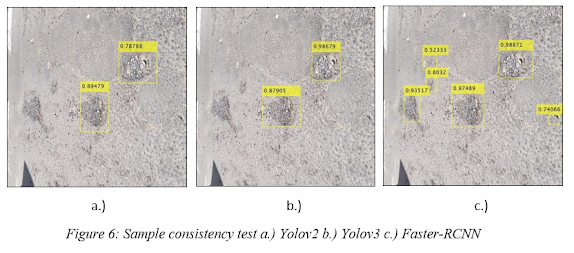
Figure 6 above expressed the consistency test over all the models. The consistency test shows how consistent the model can detect without missing the targeted object. In this test, the Fast-RCNN model was not able to detect any pothole at all. However, the rest of the models remains with diferent confidence and hit scores. Faster-RCNN has the highest hit score for this image showing a 100% hit ratio with 3 misclassifications. The 3 misclassifications could be justified as sags that may results into a pothole while the right corner was a total misclassification of a stone.

Four pothole detection models were successfully trained and evaluated with the help of computer vision and deep learning toolbox. In contrast of the models performance, a few metrics were adopted to analyze each models. The performance of each models differ a lot in different areas and must be chosen depending on the users’ desire and specifications. However, this paper has contrasted the SOA models as for Faster-RCNN to be the most precise, accurate and with the highest score. Yolov2 also have high precision, accuracy and score, but was outperformed by Faster-RCNN based on the metrics context. Whilst, when both models were subjected into video frame tests, Yolov2 outperformed Faster-RCNN with very less misclassifications. The Yolov3 model has acceptable results while Fast-RCNN had poor performance.

The video has no sound!

Video Testing the Yolov2 (left) & Yolov3 (right) model at 100 epochs

Video Testing the Fast-RCNN (left) & Faster-RCNN (right) model at 50 epochs